
Identifying a knife with Artificial Intelligence
For a fun challenge, I started learning a little bit of AI and Machine Learning. I’ve been studying the excellent Fast.AI course. This is a series of videos which takes you from zero to hero with Machine Learning for free.
As part of my learning process, I wanted to use my own dataset. I took a few days to choose a problem but my criteria were:
- A freely available dataset
- Could be used for social good
- Not overly complex for my first attempt
So after scouring Kaggle and the internet in general for a cool dataset, I stumbled upon a database of knife images which contained both positive and negative examples. With my dataset in hand, it was time to get to work!
Social Good
Unfortunately knife crime is a serious problem in the UK. In the year ending March 2018 there were around 40,100 offences involving a knife or sharp instrument in England and Wales.
I thought that by being able to recognise knives in images then there could be a potential application in crime detection and reduction and put AI to some social good.
Method
Data Structuring
Firstly I collated my data and put all of my images into a single folder with the naming pattern:
knife_1.bmp
notknife_1.bmp
The numbers are sequential: so knife_1, knife_2, etc.
Running Jupyter Notebook
Jupyter notebooks are the de-facto tool for running these datasets and I didn’t deviate from this.
Firstly I set my notebook to automatically update, and loaded my FastAI libraries:
!pip install --upgrade fastai
%reload_ext autoreload
%autoreload 2
%matplotlib inline
from fastai.vision import *
from fastai.metrics import error_rate
Next I imported my data so that my model could easily access it:
path = Path('/data/')
knives = fnames = get_image_files(path)
print(knives[:5])
I printed out a set of five of my file names to check that they were being imported effectively:
[PosixPath('/data/notknife_3198.bmp'), PosixPath('/data/notknife_2790.bmp'), PosixPath('/data/notknife_2296.bmp'), PosixPath('/data/notknife_8269.bmp'), PosixPath('/data/notknife_5795.bmp')]Next I created a regex pattern to grab the label from each of our file names to be able to classify them as a knife or not as a knife:
pat = r'/([^/]+)_\d+.bmp$'Then I leveraged one of FastAI’s functions which bundles our images together in a format suitable for computer vision:
data = (ImageDataBunch
        .from_name_re(path,
                      knives,
                      pat,
                      ds_tfms=get_transforms(),
                      size=224,
                      bs=64)
	.normalize(imagenet_stats))
So as you can see above, we have our path to access the data, our training set in the form of knives, then we ensure they are valid by applying our regex, we resize the images to a uniform 224 (a multiplier of 7 which is optimal for our RestNet data which comes later) and then we normalise the dataset.
To check this has all gone as we expected, I output 4 rows of our images as well as the two anticipated labels: knife, notknife:
data.show_batch(rows=4)
print(data.classes)
As the output I get the following:
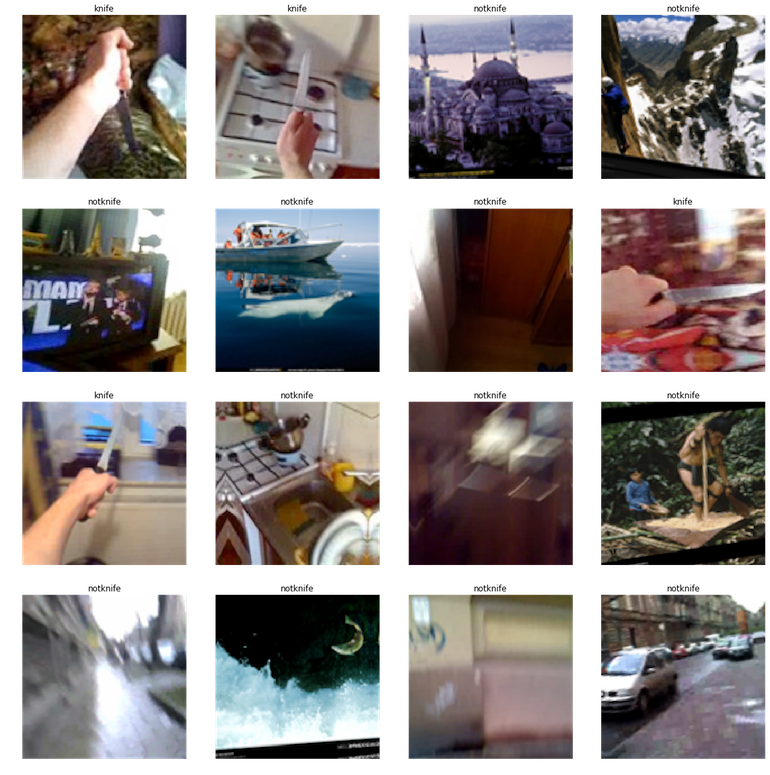
Great, so I have the images I expect and they’re correctly labelled. Now it’s time to start training my model.
Training the model
To do so, I’m using a convolutional neural network or CNN and training against resnet50 which, as its name implies is a 50 layer residual network. This allows us to use something called transfer learning which is leveraging knowledge stored in one model and apply it to another. Essentially it’s a starting point for our model.
Using Fast.AI this is extremely simple:
learn = create_cnn(data, models.resnet50, metrics=error_rate)
learn.fit_one_cycle(4)
learn.save('knives-stage-1')
As you can see above we are creating our CNN, creating a learner object from the data we provide and the model inferred from resnet. We use differential learning rates to then train the model.
Once completed, and this can take a while! We end up with something like this:
| epoch | train_loss | valid_loss | error_rate |
|---|---|---|---|
| 1 | 0.158432 | 0.063633 | 0.020894 |
| 2 | 0.020894 | 0.034570 | 0.012119 |
| 3 | 0.040913 | 0.019557 | 0.006268 |
| 4 | 0.025303 | 0.017205 | 0.005433 |
So as you can see, we start with a higher error rate and gradually reduce it from 98% accuracy to 99.5% accuracy.
So this is already great! But can we do better? Let’s figure out where our model is getting confused.
Identifying model errors
interp = ClassificationInterpretation.from_learner(learn)
interp.plot_top_losses(9)
By running the above I’m asking FastAI to interpret the results and display the top 9 incorrect guesses which returns this:

Hmm. So this makes sense looking at it with our human eyes. The tool the woman is using with a snake looks quite like a knife, and the image in the top right has terrible contrast so it’s hard to identify the blade.
Ok great, so let’s find out where our error rates starts to shoot up and see if we can improve on that:
learn.lr_find()
learn.recorder.plot()
This renders the following chart:

So we can see a strong dip towards the right of the chart before the error rate spikes again, so let’s calibrate our model to use the data from between the start of the top of the dip and where it terminates.
learn.fit_one_cycle(10, max_lr=slice(1e-03,1e-02))
learn.save('knives-stage-2')
Here we are running our training for ten cycles (or epochs) and slicing our data to fit the chart as described above.
We then receive the following:
| epoch | train_loss | valid_loss | error_rate |
|---|---|---|---|
| 1 | 0.031050 | 0.018738 | 0.005433 |
| 2 | 0.029380 | 0.040244 | 0.009611 |
| 3 | 0.040095 | 0.028016 | 0.005015 |
| 4 | 0.027003 | 0.022205 | 0.004597 |
| 5 | 0.025842 | 0.010071 | 0.001672 |
| 6 | 0.024286 | 0.039495 | 0.009193 |
| 7 | 0.012359 | 0.008150 | 0.002507 |
| 8 | 0.004851 | 0.006673 | 0.001254 |
| 9 | 0.003144 | 0.005253 | 0.001672 |
| 10 | 0.002792 | 0.004225 | 0.001672 |
So we can see a much lower error rate on our second pass, and a particularly good set of results towards the end. By the time the training has completed, we have reached an astonishing 99.84% accuracy rate!
The next steps that I will take with this is to wrap the model in an API so you can upload images and be reliably informed if a knife is present or not. I could imagine this being useful for law enforcement or security in particular but the techniques used here could easily be applied to any subject matter.
Conclusion
Hopefully you found this to be an informative read and will try and use the same techniques to generate your own computer vision applications.
This was my first time working with this technology in depth and so I’m sure there will be mistakes in my process or interpretation. Please reach out if you spot anything or think there are ways that this could be improved further. I’d love to hear!